Advent of Code 2015 - Day 9: All in a Single Night

Part 1

Description

Every year, Santa manages to deliver all of his presents in a single night.
This year, however, he has some new locations to visit; his elves have provided him the distances between every pair of locations. He can start and end at any two (different) locations he wants, but he must visit each location exactly once. What is the shortest distance he can travel to achieve this?
For example, given the following distances:

London to Dublin = 464
London to Belfast = 518
Dublin to Belfast = 141

The possible routes are therefore:

Dublin -> London -> Belfast = 982
London -> Dublin -> Belfast = 605
London -> Belfast -> Dublin = 659
Dublin -> Belfast -> London = 659
Belfast -> Dublin -> London = 605
Belfast -> London -> Dublin = 982

The shortest of these is London -> Dublin -> Belfast = 605, and so the answer is 605 in this example.
What is the distance of the shortest route?

Input

Solution

This problem is also known as traveling salesman problem, with exception, that Santa doesn't go back to the starting point. I don't have any better solution than this. First, I paste and split the input.

Then, I put those numbers into a table. Because there are eight locations, I made an 8×8 table, pairing each of them.

As you can see, the table shows all the distance between those locations, marked with numbers 1-8. There are 8! (40320) possibilities of routes taken. Or precisely, there are just half of it, because the distance of route 1-2-3-4-5-6-7-8 is the same as route 8-7-6-5-4-3-2-1. So, I made a list of all possible permutation from these  numbers, like this:

Here is the way to do it. I went to a blank sheet and paste the following formula in A1.

= IF(ROW()<=FACT(COLUMN()-1),COLUMN(),
INDIRECT(ADDRESS(ROW()-FACT(SUMPRODUCT(((ROW()-1)>=FACT(ROW($A$2:$A$10)))+0)+1),
IF(COLUMN()=(SUMPRODUCT(((ROW()-1)>=FACT(ROW($A$2:$A$10)))+0)+2),1,COLUMN()+1))))

Then, by dragging the formula to 8 columns and 40320 rows, I get the permutation I need. Next, I put another formula in seven columns (Q-X), one for each distance between two adjacent places, and sum them up. The formula in Q13 is:

=INDEX($H$4:$O$11,H13,I13)

And, finally a formula to return the smallest value of the sum of the distances:

=SMALL(X13:X40332,1)

Part 2

Description

The next year, just to show off, Santa decides to take the route with the longest distance instead.
He can still start and end at any two (different) locations he wants, and he still must visit each location exactly once.
For example, given the distances above, the longest route would be 982 via (for example) Dublin -> London -> Belfast.
What is the distance of the longest route?

Solution

For the part 2, I just need to modify the formula to get the longest route.

=LARGE(X13:X40332,1)

Read More

Advent of Code 2015 - Day 8: Matchsticks

Part 1

Description

Space on the sleigh is limited this year, and so Santa will be bringing his list as a digital copy. He needs to know how much space it will take up when stored.
It is common in many programming languages to provide a way to escape special characters in strings. For example, C, JavaScript, Perl, Python, and even PHP handle special characters in very similar ways.
However, it is important to realize the difference between the number of characters in the code representation of the string literal and the number of characters in the in-memory string itself.
For example:

• "" is 2 characters of code (the two double quotes), but the string contains zero characters.
• "abc" is 5 characters of code, but 3 characters in the string data.
• "aaa\"aaa" is 10 characters of code, but the string itself contains six "a" characters and a single, escaped quote character, for a total of 7 characters in the string data.
• "\x27" is 6 characters of code, but the string itself contains just one - an apostrophe ('), escaped using hexadecimal notation.

Santa's list is a file that contains many double-quoted string literals, one on each line. The only escape sequences used are \\ (which represents a single backslash), \" (which represents a lone double-quote character), and \x plus two hexadecimal characters (which represents a single character with that ASCII code).
Disregarding the whitespace in the file, what is the number of characters of code for string literals minus the number of characters in memory for the values of the strings in total for the entire file?
For example, given the four strings above, the total number of characters of string code (2 + 5 + 10 + 6 = 23) minus the total number of characters in memory for string values (0 + 3 + 7 + 1 = 11) is 23 - 11 = 12.

Input

Solution

Unfortunately, (as far as I know) Excel or VBA doesn't support escape string. So, I have to do it with substitute. Here is my solution.

I put this formula in B3:

=IFERROR(SUBSTITUTE(A3,MID(A3,SEARCH("\x??",A3),4),CHAR(HEX2DEC(MID(MID(A3,SEARCH("\x??",A3),4),3,2)))),A3)

This formula search for hexadecimal notation and replace it with corresponding character. I have to run it several times (column B to E) because each notation is unique. Next, in F3, I put the following:

=SUBSTITUTE(SUBSTITUTE(E3,"\"&CHAR(34),CHAR(34)),"\\","\")

The formula replace any \\ with \ and \" with ". Then, I calculate the length of these strings (the original and the modified one). For the modified one, I have to subtract it by 2 for opening and closing double quotes.

From calculating this length of stings, I can also know whether I still need another column for running the first formula or not. Subtracting the length of original string and the modified one and summing them give me the desired output.

Part 2

Description

Now, let's go the other way. In addition to finding the number of characters of code, you should now encode each code representation as a new string and find the number of characters of the new encoded representation, including the surrounding double quotes.
For example:

• "" encodes to "\"\"", an increase from 2 characters to 6.
• "abc" encodes to "\"abc\"", an increase from 5 characters to 9.
• "aaa\"aaa" encodes to "\"aaa\\\"aaa\"", an increase from 10 characters to 16.
• "\x27" encodes to "\"\\x27\"", an increase from 6 characters to 11.

Your task is to find the total number of characters to represent the newly encoded strings minus the number of characters of code in each original string literal. For example, for the strings above, the total encoded length (6 + 9 + 16 + 11 = 42) minus the characters in the original code representation (23, just like in the first part of this puzzle) is 42 - 23 = 19.

Solution

For the part 2, I just need to modify the formula, count the length of the strings, subtract them from the length of the original ones, and sum up them. The formula looks like this.

=SUBSTITUTE(SUBSTITUTE(A3,"\","\\"),CHAR(34),"\"&CHAR(34))

Read More

Advent of Code 2015 - Day 7: Some Assembly Required

Part 1

Description

This year, Santa brought little Bobby Tables a set of wires and bitwise logic gates! Unfortunately, little Bobby is a little under the recommended age range, and he needs help assembling the circuit.
Each wire has an identifier (some lowercase letters) and can carry a 16-bit signal (a number from 0 to 65535). A signal is provided to each wire by a gate, another wire, or some specific value. Each wire can only get a signal from one source, but can provide its signal to multiple destinations. A gate provides no signal until all of its inputs have a signal.
The included instructions booklet describes how to connect the parts together: x AND y -> z means to connect wires x and y to an AND gate, and then connect its output to wire z.
For example:

• 123 -> x means that the signal 123 is provided to wire x.
• x AND y -> z means that the bitwise AND of wire x and wire y is provided to wire z.
• p LSHIFT 2 -> q means that the value from wire p is left-shifted by 2 and then provided to wire q.
• NOT e -> f means that the bitwise complement of the value from wire e is provided to wire f.

Other possible gates include OR (bitwise OR) and RSHIFT (right-shift). If, for some reason, you'd like to emulate the circuit instead, almost all programming languages (for example, C, JavaScript, or Python) provide operators for these gates.
For example, here is a simple circuit:

123 -> x
456 -> y
x AND y -> d
x OR y -> e
x LSHIFT 2 -> f
y RSHIFT 2 -> g
NOT x -> h
NOT y -> i

After it is run, these are the signals on the wires:

d: 72
e: 507
f: 492
g: 114
h: 65412
i: 65079
x: 123
y: 456

In little Bobby's kit's instructions booklet (provided as your puzzle input), what signal is ultimately provided to wire a?

Input

Solution

Today's problem is quite difficult for me. But it only made me more challenged. At first, I was thinking of using VBA code to automate the whole things. But, running the code takes forever, maybe because I don't know how to break the loop. But, then I realize, that this puzzle can be done also with matching and sorting. So, in my Excel file below, I split the input into 5 parts: two variables, one operator, the -> and variable 3 (the result).

The column G is for sorting those five columns. First I put this formula in the column (row 1 to 342, respectively):

=SUM(IF(B4="",1,0),IF(C4="",1,0),ISNUMBER(D4)))

This formula basically checks if the first variable and the operator is empty and the second is a number. Those meeting these conditions (signal in variable 3 is provided by variable 2) will give the sum of three. By sorting the columns (B-G) with value of G from largest to smallest, I can put those with numeric variable 2 in the top row. Then, I put this array formula in G6 (which has value less than 2):

=SUM(IF($B6="",1,0),IF($D6=$F$4:INDIRECT(ADDRESS(ROW(G$5),6)),1,0))+SUM(IF(ISNUMBER($B6),1,0),IF($D6=$F$4:INDIRECT(ADDRESS(ROW(G$5),6)),1,0))+SUM(IF(ISNUMBER($D6),1,0),IF($B6=$F$4:INDIRECT(ADDRESS(ROW(G$5),6)),1,0))

The formula again checks if any variable 1 and variable 2 matches those already declared variable 3 (c and b respectively). Only if both match, or one variable match and another one is a number, that it will give values of one (true). Again, by sorting the columns (B-G) with value of G from largest to smallest, I can put those meeting the condition in the cells below the already declared variables. I repeat the process (with the help of a Macro) until the last row (G342). And, as I already guess, there is the desired output (signal provided to a) in the last row.

Now, to give value to variables 3, I made a custom function, called Operate:

Function Operate(a, b, c) As Double
If c = "AND" Then
    Operate = WorksheetFunction.Bitand(a, b)
ElseIf c = "OR" Then
    Operate = WorksheetFunction.Bitor(a, b)
ElseIf c = "LSHIFT" Then
    Operate = WorksheetFunction.Bitlshift(a, b)
ElseIf c = "RSHIFT" Then
    Operate = WorksheetFunction.Bitrshift(a, b)
ElseIf c = "NOT" Then
    Operate = 65535 - b
ElseIf c = "" Then
    Operate = b
End If
End Function

This function, basically put together all bitwise function needed (BITAND, BITOR, BITLSHIFT, and BITRSHIFT), with addition of BITNOT (there is no such Excel function) and direct signal. Therefore, I just need to put this formula in column H:

=Operate(IFERROR(INDEX($H$4:$H5,MATCH(B6,$F$4:$F$342,0)),B6),IFERROR(INDEX($H$4:$H5,MATCH(D6,$F$4:$F$342,0)),D6),C6)

The function IFERROR is needed because sometimes the variable (1 or 2) doesn't match with variable 3 and the formula returns an error value. The output is what I get in the last row.

Part 2

Description

Now, take the signal you got on wire a, override wire b to that signal, and reset the other wires (including wire a). What new signal is ultimately provided to wire a?

Solution

For the part 2, I put the value of  b from the part 1 in the place of 44430 and calculate a using the same formula as above.

Read More

Advent of Code 2015 - Day 6: Probably a Fire Hazard

Part 1

Description

Because your neighbors keep defeating you in the holiday house decorating contest year after year, you've decided to deploy one million lights in a 1000x1000 grid.
Furthermore, because you've been especially nice this year, Santa has mailed you instructions on how to display the ideal lighting configuration.
Lights in your grid are numbered from 0 to 999 in each direction; the lights at each corner are at 0,0, 0,999, 999,999, and 999,0. The instructions include whether to turn on, turn off, or toggle various inclusive ranges given as coordinate pairs. Each coordinate pair represents opposite corners of a rectangle, inclusive; a coordinate pair like 0,0 through 2,2 therefore refers to 9 lights in a 3x3 square. The lights all start turned off.
To defeat your neighbors this year, all you have to do is set up your lights by doing the instructions Santa sent you in order.
For example:

• turn on 0,0 through 999,999 would turn on (or leave on) every light.
• toggle 0,0 through 999,0 would toggle the first line of 1000 lights, turning off the ones that were on, and turning on the ones that were off.
• turn off 499,499 through 500,500 would turn off (or leave off) the middle four lights.

After following the instructions, how many lights are lit?

Input

Solution

For this problem, at first I thought of making a grid of 1000*1000 cells, marked with coordinates of (0,0) through (999,999). But, then it will be long to make a calculation in such vast area. So, I decided to use VBA, reading the input, and constructing the grid in a two dimensional array. Here is the split input in Excel.

And, the code:

Sub Hazard3()
    Dim c, x0, y0, x1, y1, x2, y2, rows As Integer
    Dim map(0 To 999, 0 To 999) As Variant
    Dim action As String
    ActiveSheet.Range("h3").Select
    x0 = 11
    y0 = 11
Start:
    ActiveCell.Offset(1, 0).Select
    rows = ActiveCell.Row
    x1 = Cells(rows, 3).Value
    y1 = Cells(rows, 4).Value
    x2 = Cells(rows, 6).Value
    y2 = Cells(rows, 7).Value
    action = Cells(rows, 2).Value
    If IsEmpty(Cells(rows, 3)) Then
        GoTo Finish
        Else
        If action = "turnon" Then
                For c = x1 To x2
                For d = y1 To y2
                map(c, d) = 1
                Next d
                Next c
            ElseIf action = "turnoff" Then
                For c = x1 To x2
                For d = y1 To y2
                map(c, d) = 0
                Next d
                Next c
            Else
                For c = x1 To x2
                For d = y1 To y2
                map(c, d) = (map(c, d) + 1) Mod 2
                Next d
                Next c
        End If
    End If
    ActiveSheet.Cells(rows, 7).Select
    GoTo Start
Finish:
ActiveSheet.Cells(3, 10).Select
ActiveCell.Value = Application.WorksheetFunction.Sum(map)
End Sub

This code basically modify the value of corresponding array (map) according to the input value and the instruction (toggle, turn on or turn off) and finally sum up the array.

Part 2

Description

You just finish implementing your winning light pattern when you realize you mistranslated Santa's message from Ancient Nordic Elvish.
The light grid you bought actually has individual brightness controls; each light can have a brightness of zero or more. The lights all start at zero.
The phrase turn on actually means that you should increase the brightness of those lights by 1.
The phrase turn off actually means that you should decrease the brightness of those lights by 1, to a minimum of zero.
The phrase toggle actually means that you should increase the brightness of those lights by 2.
What is the total brightness of all lights combined after following Santa's instructions?
For example:

• turn on 0,0 through 0,0 would increase the total brightness by 1.
• toggle 0,0 through 999,999 would increase the total brightness by 2000000.

Solution

For the part 2, only the instruction is changed. So, I modified the code into this:

Sub Hazard2()
    Dim c, x0, y0, x1, y1, x2, y2, rows As Integer
    Dim map(0 To 999, 0 To 999) As Variant
    Dim action As String
    ActiveSheet.Range("h3").Select
    x0 = 11
    y0 = 11
Start:
    ActiveCell.Offset(1, 0).Select
    rows = ActiveCell.Row
    x1 = Cells(rows, 3).Value
    y1 = Cells(rows, 4).Value
    x2 = Cells(rows, 6).Value
    y2 = Cells(rows, 7).Value
    action = Cells(rows, 2).Value
    If IsEmpty(Cells(rows, 3)) Then
        GoTo Finish
        Else
        If action = "turnon" Then
                For c = x1 To x2
                For d = y1 To y2
                map(c, d) = map(c, d) + 1
                Next d
                Next c
            ElseIf action = "turnoff" Then
                For c = x1 To x2
                For d = y1 To y2
                If map(c, d) > 0 Then
                map(c, d) = map(c, d) - 1
                End If
                Next d
                Next c
            Else
                For c = x1 To x2
                For d = y1 To y2
                map(c, d) = map(c, d) + 2
                Next d
                Next c
        End If
    End If
    ActiveSheet.Cells(rows, 7).Select
    GoTo Start
Finish:
ActiveSheet.Cells(5, 10).Select
ActiveCell.Value = Application.WorksheetFunction.Sum(map)
End Sub

Read More

Advent of Code 2015 - Day 5: Doesn't He Have Intern-Elves For This?

Part 1

Description

Santa needs help figuring out which strings in his text file are naughty or nice.
A nice string is one with all of the following properties:

• It contains at least three vowels (aeiou only), like aei, xazegov, or aeiouaeiouaeiou.
• It contains at least one letter that appears twice in a row, like xx, abcdde (dd), or aabbccdd (aa, bb, cc, or dd).
• It does not contain the strings ab, cd, pq, or xy, even if they are part of one of the other requirements.

For example:

• ugknbfddgicrmopn is nice because it has at least three vowels (u...i...o...), a double letter (...dd...), and none of the disallowed substrings.
• aaa is nice because it has at least three vowels and a double letter, even though the letters used by different rules overlap.
• jchzalrnumimnmhp is naughty because it has no double letter.
• haegwjzuvuyypxyu is naughty because it contains the string xy.
• dvszwmarrgswjxmb is naughty because it contains only one vowel.

How many strings are nice?

Input

Solution

So, there are three conditions to be met for a string to be nice. Therefore, in my Excel file, after putting the input in the leftmost column, I put these condition in the adjacent columns.

Column C is for counting the number of vowels, using this formula:

=LEN(A3)-LEN(SUBSTITUTE(SUBSTITUTE(SUBSTITUTE(SUBSTITUTE(SUBSTITUTE(A3,"a",""),"e",""),"i",""),"o",""),"u",""))

Column D is for counting any double letter, using this array formula:

=SUM(IF(MID($A3,(ROW(INDIRECT("1:"&LEN($A3)))),1)=MID($A3,1+(ROW(INDIRECT("1:"&LEN($A3)))),1),1,0))

Column E is for counting any special condition above, using this formula:

=LEN(A3)-LEN(SUBSTITUTE(SUBSTITUTE(SUBSTITUTE(SUBSTITUTE(A3,"ab",""),"cd",""),"pq",""),"xy",""))

Now, what is left is counting how many strings fulfill these conditions.

Part 2

Description

Realizing the error of his ways, Santa has switched to a better model of determining whether a string is naughty or nice. None of the old rules apply, as they are all clearly ridiculous.
Now, a nice string is one with all of the following properties:

• It contains a pair of any two letters that appears at least twice in the string without overlapping, like xyxy (xy) or aabcdefgaa (aa), but not like aaa (aa, but it overlaps).
• It contains at least one letter which repeats with exactly one letter between them, like xyx, abcdefeghi (efe), or even aaa.

For example:

• qjhvhtzxzqqjkmpb is nice because is has a pair that appears twice (qj) and a letter that repeats with exactly one letter between them (zxz).
• xxyxx is nice because it has a pair that appears twice and a letter that repeats with one between, even though the letters used by each rule overlap.
• uurcxstgmygtbstg is naughty because it has a pair (tg) but no repeat with a single letter between them.
• ieodomkazucvgmuy is naughty because it has a repeating letter with one between (odo), but no pair that appears twice.

How many strings are nice under these new rules?

Solution

For the part two, the conditions have changed. So I just added two more columns. Column H is for counting instances of two letters appear twice, using array formula:

=SUM(LEN(A3)-LEN(SUBSTITUTE($A3,MID($A3,(ROW(INDIRECT("1:"&LEN($A3)-1))),2),"")))

If the result is 30, it means there is no instance of two letters appear twice. Each string in the input is exactly 16 character long. So, there will be 15 pairings. When one of these pairs (for example, xy) matches with itself, the formula will return a value of two (and total of 30 for the whole string). When it matches another pair, the formula will return another value of two. So, when the result is more than 30, it means that string contains two letters that appear more than once.
Column I is for counting if there is any letter which repeats with exactly one letter between them, using array formula:

=SUM(IF(MID($A3,(ROW(INDIRECT("1:"&LEN($A3)))),1)=MID($A3,2+(ROW(INDIRECT("1:"&LEN($A3)))),1),1,0))

And again, all I need is counting how many strings fulfill these conditions.

Read More

Advent of Code 2015 - Day 4: The Ideal Stocking Stuffer

Part 1

Description

Santa needs help mining some AdventCoins (very similar to bitcoins) to use as gifts for all the economically forward-thinking little girls and boys.
To do this, he needs to find MD5 hashes which, in hexadecimal, start with at least five zeroes. The input to the MD5 hash is some secret key (your puzzle input, given below) followed by a number in decimal. To mine AdventCoins, you must find Santa the lowest positive number (no leading zeroes:  1, 2, 3, ...) that produces such a hash.
For example:

• If your secret key is abcdef, the answer is 609043, because the MD5 hash of abcdef609043 starts with five zeroes (000001dbbfa...), and it is the lowest such number to do so.
• If your secret key is pqrstuv, the lowest number it combines with to make an MD5 hash starting with five zeroes is 1048970; that is, the MD5 hash of pqrstuv1048970 looks like 000006136ef....

Input

Solution

The input for this puzzle is relatively short. But, the difficulty to obtain the answer is incredibly painful. Firstly, because I don't really know what on earth MD5 hash is (even after reading about it) and how it is obtained. Secondly, MS Excel doesn't have a ready-to-use function to obtain MD5 hash value. So, my Excel only looked like this:

Those two buttons are for running the Macros, something I added later.
After reading and searching for few hours, I found this file in this website. But, after carefully examined it, I decided not to use it because it only supported finding the MD5 hash value for a string in one cell. Modifying it to serve my purpose also seemed impossible because I don't understand a dime about it. Therefore I tried to find a VBA code for generating that MD5 hash and found it here. The code is quite long, so that I will not post it here.
Now, after found the code, all left is to add a Macro to run the code until the hash reached the first value starting with five zeroes. Here is my Macro:

Sub Hitung()
    Dim input4, output4 As String
    Dim i As Double
    
    i = 0
Start:
    input4 = "iwrupvqb" & i
    output = MD5Hash(input4)
    Debug.Print output
    i = i + 1
    If Mid(output, 1, 5) = "00000" Then
        GoTo Finish
    Else
        GoTo Start
    End If
Finish:
    ActiveSheet.Range("b4").Select
    ActiveCell.Value = i - 1
End Sub

Part 2

Description

Now find one that starts with six zeroes.

Solution

And, the macro for the second part:

Sub Hitung2()
    Dim input4, output4 As String
    Dim i As Double
    
    i = 0
Start:
    input4 = "iwrupvqb" & i
    output = MD5Hash(input4)
    Debug.Print output
    i = i + 1
    If Mid(output, 1, 6) = "000000" Then
        GoTo Finish
    Else
        GoTo Start
    End If
Finish:
    ActiveSheet.Range("b5").Select
    ActiveCell.Value = i - 1
End Sub

Read More

Advent of Code 2015 - Day 3: Perfectly Spherical Houses in a Vacuum

Part 1

Description

Santa is delivering presents to an infinite two-dimensional grid of houses.
He begins by delivering a present to the house at his starting location, and then an elf at the North Pole calls him via radio and tells him where to move next. Moves are always exactly one house to the north (^), south (v), east (>), or west (<). After each move, he delivers another present to the house at his new location.
However, the elf back at the north pole has had a little too much eggnog, and so his directions are a little off, and Santa ends up visiting some houses more than once. How many houses receive at least one present?
For example:

• > delivers presents to 2 houses: one at the starting location, and one to the east.
• ^>v< delivers presents to 4 houses in a square, including twice to the house at his starting/ending location.
• ^v^v^v^v^v delivers a bunch of presents to some very lucky children at only 2 houses.

Input

Solution

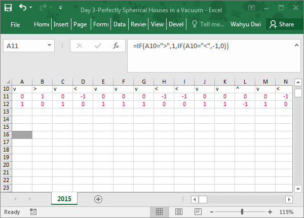
For this day's puzzle, I decided to use VBA. It's because I don't think it will be possible to solve it with just formulas. But, first I have to split and translate this input into readable variables, i.e. offsets in Excel. So, going north is translated into offset (-1,0) or one column upward, etc.

Then, I write a VBA code that looks like this:

Sub Perfectly()
    Dim x, y, posx, posy, lastx, lasty, startx, starty As Integer
    Dim lastpos, curpos As Range
    
    ActiveSheet.Range("a11").Select
    x = ActiveCell.Value
    ActiveCell.Offset(1, 0).Select
    y = ActiveCell.Value
    lasty = ActiveCell.Row
    lastx = ActiveCell.Column
    ActiveSheet.Cells(60, 100).Select
    ActiveCell.Value = ActiveCell.Value + 1
Start:
    ActiveCell.Offset(y, x).Select
    ActiveCell.Value = ActiveCell.Value + 1
    posy = ActiveCell.Row
    posx = ActiveCell.Column
    ActiveSheet.Cells(lasty, lastx).Select
    ActiveCell.Offset(-1, 1).Select
If IsEmpty(ActiveCell.Value) = False Then
    x = ActiveCell.Value
    ActiveCell.Offset(1, 0).Select
    y = ActiveCell.Value
    lasty = ActiveCell.Row
    lastx = ActiveCell.Column
    ActiveSheet.Cells(posy, posx).Select
    GoTo Start
    Else: GoTo Ended
End If
Ended:
End Sub

Again, I am not a programmer, only a hobbyist. Therefore I didn't wrote this code for its speed. For me, as long as it works, it's OK. So, let me explain a bit about the code. Line 5-10 are practically for reading the translated input. Line 11-12 do the starting location, by adding value +1 to that location. The Loop between Start: and Ended: is doing the rest, moving left and right, up and down, and every time adding value +1. In the end, I counted (not sum!) all the filled cells, using:

=COUNTIF(A17:EH108,">0")

Part 2

Description

The next year, to speed up the process, Santa creates a robot version of himself, Robo-Santa, to deliver presents with him.

Santa and Robo-Santa start at the same location (delivering two presents to the same starting house), then take turns moving based on instructions from the elf, who is eggnoggedly reading from the same script as the previous year.

This year, how many houses receive at least one present?

For example:

• ^v delivers presents to 3 houses, because Santa goes north, and then Robo-Santa goes south.
• ^>v< now delivers presents to 3 houses, and Santa and Robo-Santa end up back where they started.
• ^v^v^v^v^v now delivers presents to 11 houses, with Santa going one direction and Robo-Santa going the other.

Solution

Now, for the part two, the VBA code is similar to the one in the part one, only there has to be two different parts reading inputs and moving independently. The code I made looks like this:

Sub Perfectly2()
    Dim x, y, posax, posay, posby, posbx, lastx, lasty, startx, starty As Integer
    Dim lastpos, curpos As Range
    
    ActiveSheet.Range("a11").Select
    x = ActiveCell.Value
    ActiveCell.Offset(1, 0).Select
    y = ActiveCell.Value
    lasty = ActiveCell.Row
    lastx = ActiveCell.Column
    ActiveSheet.Cells(260, 100).Select
    ActiveCell.Value = ActiveCell.Value + 1
    ActiveCell.Offset(y, x).Select
    ActiveCell.Value = ActiveCell.Value + 1
    posay = ActiveCell.Row
    posax = ActiveCell.Column
    ActiveSheet.Cells(lasty, lastx).Select
    ActiveCell.Offset(-1, 1).Select
    x = ActiveCell.Value
    ActiveCell.Offset(1, 0).Select
    y = ActiveCell.Value
    lasty = ActiveCell.Row
    lastx = ActiveCell.Column
    ActiveSheet.Cells(260, 100).Select
    ActiveCell.Offset(y, x).Select
    ActiveCell.Value = ActiveCell.Value + 1
    posby = ActiveCell.Row
    posbx = ActiveCell.Column
    ActiveSheet.Cells(lasty, lastx).Select
    ActiveCell.Offset(-1, 1).Select
Start:
If IsEmpty(ActiveCell.Value) = False Then
    x = ActiveCell.Value
    ActiveCell.Offset(1, 0).Select
    y = ActiveCell.Value
    lasty = ActiveCell.Row
    lastx = ActiveCell.Column
    ActiveSheet.Cells(posay, posax).Select
    ActiveCell.Offset(y, x).Select
    ActiveCell.Value = ActiveCell.Value + 1
    posay = ActiveCell.Row
    posax = ActiveCell.Column
    ActiveSheet.Cells(lasty, lastx).Select
    ActiveCell.Offset(-1, 1).Select
    x = ActiveCell.Value
    ActiveCell.Offset(1, 0).Select
    y = ActiveCell.Value
    lasty = ActiveCell.Row
    lastx = ActiveCell.Column
    ActiveSheet.Cells(posby, posbx).Select
    ActiveCell.Offset(y, x).Select
    ActiveCell.Value = ActiveCell.Value + 1
    posby = ActiveCell.Row
    posbx = ActiveCell.Column
    ActiveSheet.Cells(lasty, lastx).Select
    ActiveCell.Offset(-1, 1).Select
    GoTo Start
    Else: GoTo Ended
End If
Ended:
End Sub

And, finally same formula as above to count all filled cells.

Read More

Advent of Code 2015 - Day 2: I Was Told There Would Be No Math

Part 1

Description

The elves are running low on wrapping paper, and so they need to submit an order for more. They have a list of the dimensions (length l, width w, and height h) of each present, and only want to order exactly as much as they need.

Fortunately, every present is a box (a perfect right rectangular prism), which makes calculating the required wrapping paper for each gift a little easier: find the surface area of the box, which is 2*l*w + 2*w*h + 2*h*l. The elves also need a little extra paper for each present: the area of the smallest side.

For example:

• A present with dimensions 2x3x4 requires 2*6 + 2*12 + 2*8 = 52 square feet of wrapping paper plus 6 square feet of slack, for a total of 58 square feet.
• A present with dimensions 1x1x10 requires 2*1 + 2*10 + 2*10 = 42 square feet of wrapping paper plus 1 square foot of slack, for a total of 43 square feet.

All numbers in the elves' list are in feet. How many total square feet of wrapping paper should they order?

Input

Solution

For this day's puzzle, I put the input (1000 of them) in the leftmost column. Then, I split them up into three parts: length, width, and height. Then to calculate the wrapping paper needed, i use this formula and sum up the result.

=SUM(3*SMALL(C4:E4,1)*SMALL(C4:E4,2),2*SMALL(C4:E4,1)*SMALL(C4:E4,3),2*SMALL(C4:E4,3)*SMALL(C4:E4,2))

 

Basically, the formula define the smallest, the second smallest and the largest among the three parts. Then it calculates the surface area and extra wrapping paper by multiplying the two smallest area with three and two others with two and sum the result. Finally, I sum up all the wrapping paper needed for each present.

Part 2

Description

The elves are also running low on ribbon. Ribbon is all the same width, so they only have to worry about the length they need to order, which they would again like to be exact.

The ribbon required to wrap a present is the shortest distance around its sides, or the smallest perimeter of any one face. Each present also requires a bow made out of ribbon as well; the feet of ribbon required for the perfect bow is equal to the cubic feet of volume of the present. Don't ask how they tie the bow, though; they'll never tell.

For example:

• A present with dimensions 2x3x4 requires 2+2+3+3 = 10 feet of ribbon to wrap the present plus 2*3*4 = 24 feet of ribbon for the bow, for a total of 34 feet.
• A present with dimensions 1x1x10 requires 1+1+1+1 = 4 feet of ribbon to wrap the present plus 1*1*10 = 10 feet of ribbon for the bow, for a total of 14 feet.

How many total feet of ribbon should they order?

Solution

Now, for the part two,using this formula,

=2*SMALL(C4:E4,1)+2*SMALL(C4:E4,2)+C4*D4*E4

I can easily get the smallest perimeter and the volume.

Read More